The standard advice about LLM inference is that decoding is limited by memory bandwidth. Every new token means reading all of the model’s weights from GPU memory, so the speed limit is how fast you can stream bytes. I built nanoserve, an inference server written from scratch, expecting to optimise for exactly that. The first careful measurement said I was optimising the wrong thing.
The number that didn’t fit
Qwen2.5-0.5B in fp16 is 943 MiB of weights, and my laptop’s RTX 4060 sustains about 210 to 226 GB/s on a plain memory copy. If memory were the limit, one decode step at batch size 1 should take about 4.5 ms.
| Measure | Windows 11 | WSL2 Ubuntu |
|---|---|---|
| Memory-bandwidth floor per step | ~4.5 ms | ~4.5 ms |
| Actual batch-1 step (eager transformers) | 23.7 ms | 16.6 ms |
| Cost of launching one small kernel | 7.8–15 µs | 6.8–9.2 µs |
| GPU utilisation during decode | 18% | 22% |
The step was four to five times slower than the bandwidth floor. Profiling showed why: the GPU was busy for only about a fifth of each step. The rest of the time it sat idle while the CPU issued the next of roughly 1,000 to 1,350 small kernels.
GPU computing GPU idle, waiting for the CPU to launch the next kernel
The tell: batching was almost free
If most of each step is a fixed launch cost, a bigger batch should cost almost nothing extra. That is exactly what happened. Step time went from 28 ms at batch 1 to 34 ms at batch 32, so throughput went from 35.5 to 941.8 tokens per second: a 26× gain for 20% more time per step.
I blamed Windows first, and I was wrong
My first theory was the Windows display driver model (WDDM), which routes kernel launches through the operating system’s scheduler. I predicted Linux would be much faster. The measurements didn’t back that up:
- Two consecutive runs of the same Linux setup measured the small-kernel cost at 6.8 µs and 9.2 µs. That 35% spread overlaps the Windows range.
- The two setups also ran different PyTorch builds, which changed the number of device ops per step from 1,350 to 1,014 for identical model code. That is a library difference, not an OS one.
- Utilisation was 18% against 22%. Both were overhead-bound.
On this hardware, the number of kernels is what moves decode time. The operating system is not.
What I changed because of it
Once the bottleneck was clear, every change that paid off was one that cut the number of ops per step:
| Change | Why it mattered here |
|---|---|
| RoPE cos/sin computed once per step | Positions are the same in all 24 layers; the old code built 48 identical tensors per step |
| Fused RMSNorm | Replaced an 8-kernel hand-written norm used at 48 places per step |
| Grouped-query attention inside SDPA | Stopped materialising a 7× expanded copy of K and V |
| One pinned host-to-device copy for step metadata | Was six separate small transfers per step |
Together with a faster way of mapping tokens to cache slots, these took the batch-1 step from 33.7 ms to 28.2 ms, 16% faster.
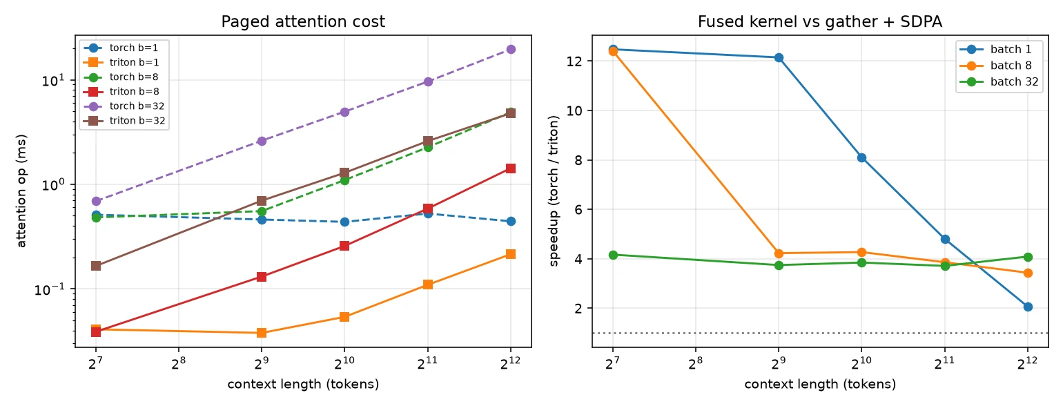
Then the fused Triton paged-attention kernel replaced about ten ops per layer with one. Device ops per step fell from 1,014 to 682, GPU utilisation at batch 32 rose from 23% to 36%, and nanoserve clearly beat eager transformers for the first time: 1.23× at batch 8.
Four measurements that lied first
Before any of these numbers could be trusted, four bugs in the measurement itself had to go. Each one produced a plausible-looking wrong answer.
- Clock ramp. The GPU idles at 210 MHz and boosts to 2,595 MHz. Whatever ran first was measured cold, which once produced “batch 32 is faster than batch 1” and a fake 3.4× win. Now there are 8 seconds of sustained work before measuring, repeated before every row.
- Double-counted kernels. The profiler attributes time to both an op and its kernel. Summing both reported 166% GPU utilisation.
- Mismatched runs. Busy time from a profiled run was being divided by wall time from an unprofiled one.
- Noise. Every configuration is now timed twice and flagged if the runs disagree by more than 15%.
Where this leaves nanoserve
Against vLLM in its strongest setup (torch.compile plus CUDA graphs), on the same GPU and the same requests, the honest comparison is:
| Server | Output tokens/s | vs vLLM |
|---|---|---|
| vLLM, compiled with CUDA graphs | 2,103.5 | 1.00× |
| nanoserve, continuous batching + Triton | 663.0 | 0.32× |
| Static batching, best batch size | 236.9 | 0.11× |
The biggest part of that gap is the same story. vLLM captures its decode step as CUDA graphs once and replays them, while nanoserve re-issues around 680 kernels every step from Python. So the next change is CUDA graphs for decode. The shapes are static, so the step can be captured once and replayed. That attacks the time spent waiting, which is still most of each step, instead of the time spent working.
The takeaway
Measure the shape of the bottleneck on your own hardware before optimising for it. “Decode is memory-bound” may well hold for a large model on a datacenter GPU. For a 0.5B model on a laptop GPU, the real step took four to five times longer than the memory floor, and the gap was all launch overhead.